Graph Databases — AGH (GitHub)

AGH · Databases II · 2026

GraphDatabases

format 90 min lecture + 90 min lab

stack Neo4j · Cypher · Fraud dataset

prereqs SQL · relational model

Block 00

Relational databases a quick recap

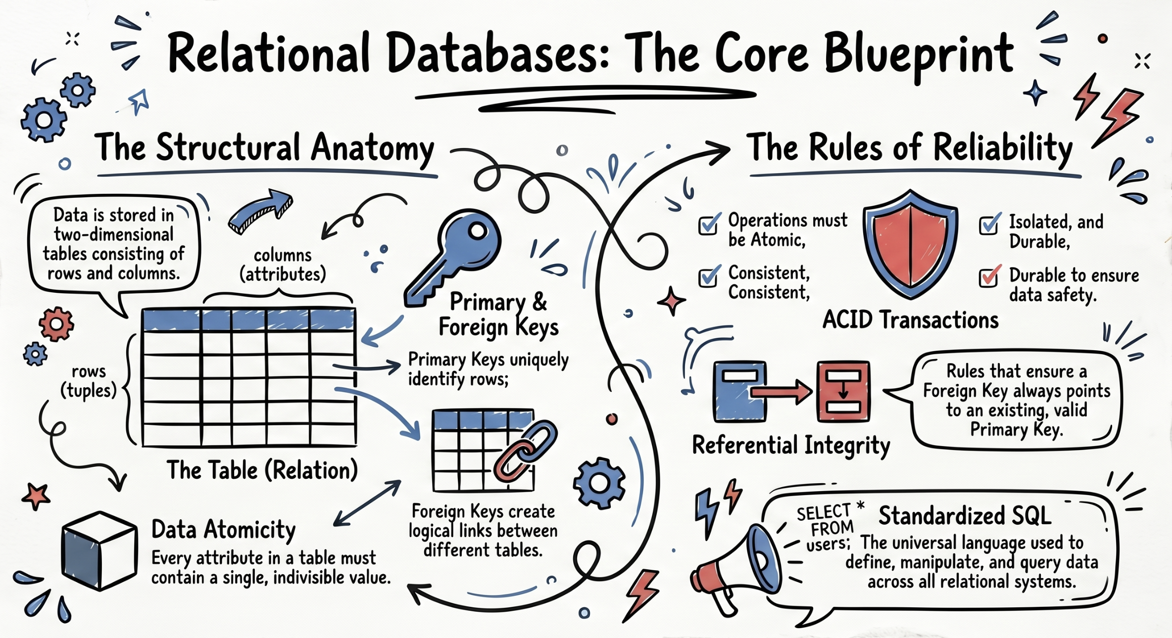
Tables with rows and columns
ACID transactions guarantee
Normalized schema design
SQL for queries and updates
Foreign keys for relationships

00

Block 00 · Relational recap

The relational model in three assumptions

Data is tabular. Every entity fits into rows and columns with a fixed schema.
Relationships are computed at query time by matching values — the JOIN operation.
Set-based operations. SQL operates on entire sets of rows, not individual records.

Edgar Codd, 1970. Dominant for 50+ years — for good reason.
Extraordinarily powerful for reporting, transactions, aggregation.

the join model — one hop

-- Users and their posts
SELECT u.name, p.title
FROM   users u
JOIN   posts p ON p.user_id = u.id;

One JOIN: fast, readable, efficient.
The engine is optimised for exactly this.

Block 00 · Relational recap → transition

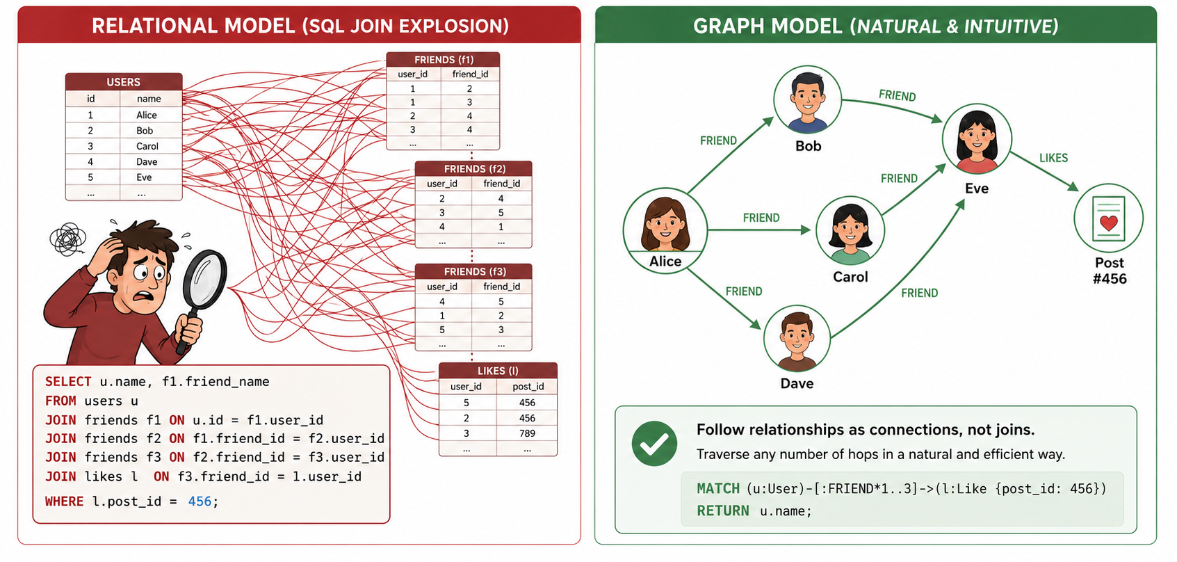
What happens when you need to follow a JOIN not once, but many times — across a chain of unknown depth?

The irony of relational databases

"For several decades, developers have tried to accommodate connected, semi-structured datasets inside relational databases. But whereas relational databases were initially designed to codify paper forms and tabular structures — something they do exceedingly well — they struggle when attempting to model the adhoc, exceptional relationships that crop up in the real world. Ironically, relational databases deal poorly with relationships."

Graph Databases — Ian Robinson, Jim Webber, Emil Eifrem

Block 01

The problem with relational
databases for connected data

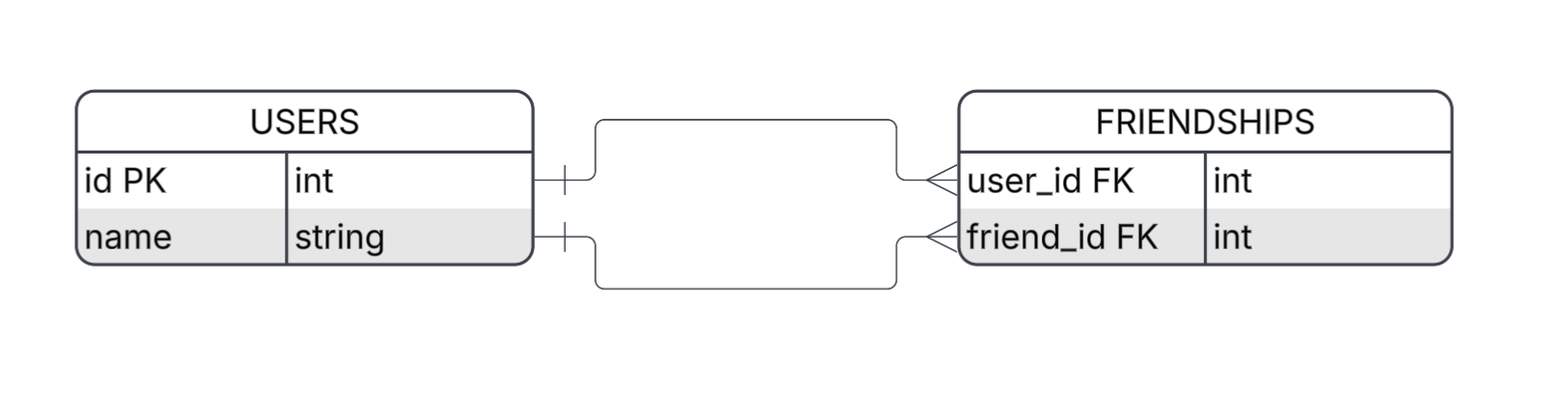
Scenario: A social network.
Data model: Two tables — Users and Friendships.
Users stores user information.
Friendships stores connections between users.
Question: "Who are Alice's friends?"

01

Block 01 · SQL escalation

The schema

CREATE TABLE users (
  id   INT PRIMARY KEY,
  name VARCHAR(100)
);
CREATE TABLE friendships (
  user_id   INT REFERENCES users(id),
  friend_id INT REFERENCES users(id),
  PRIMARY KEY (user_id, friend_id)
);

Alice ── Bob ── Dave ── Frank
  └── Carol ── Eve

1 hop — "who are Alice's friends?"

SELECT u.name AS friend
FROM   friendships f
JOIN   users u ON u.id = f.friend_id
WHERE  f.user_id = 1;

Result: Bob, Carol · Clean. 1 JOIN. Fast.

Block 01 · SQL escalation · after 1-hop

Now ask: "Who do Alice's friends know?"

Block 01 · SQL escalation

2 hops — friends of friends

"Who are the friends of Alice's friends — people Alice might know?"

Result: Dave, Eve
But: 2 JOINs + NOT IN subquery + 2 exclusion conditions.
The query now requires explanation.

postgresql — 2 hops

SELECT DISTINCT u2.name AS fof
FROM   friendships f1
JOIN   friendships f2
  ON   f2.user_id = f1.friend_id
JOIN   users u2
  ON   u2.id = f2.friend_id
WHERE  f1.user_id = 1
  AND  f2.friend_id != 1
  AND  f2.friend_id NOT IN (
    SELECT friend_id
    FROM   friendships
    WHERE  user_id = 1
  );

Block 01 · SQL escalation

3 hops — wider recommendations

"Who is three hops away from Alice?"

3 JOINs.
2 NOT IN subqueries — the second is itself a 2-hop query.
The query is longer than this paragraph.

postgresql — 3 hops (abridged)

SELECT DISTINCT u3.name AS third
FROM   friendships f1
JOIN   friendships f2 ON f2.user_id = f1.friend_id
JOIN   friendships f3 ON f3.user_id = f2.friend_id
JOIN   users u3       ON u3.id = f3.friend_id
WHERE  f1.user_id = 1
  AND  f3.friend_id != 1
  AND  f3.friend_id NOT IN (
    SELECT friend_id FROM friendships
    WHERE  user_id = 1
  )
  AND  f3.friend_id NOT IN (
    SELECT f2i.friend_id
    FROM   friendships f1i
    JOIN   friendships f2i
      ON   f2i.user_id = f1i.friend_id
    WHERE  f1i.user_id = 1
  );

Block 01 · SQL escalation · after 3-hop query

What does a new team member feel when they open this file at 2am during an incident?

Block 01

01

Block 01 · SQL escalation — the numbers

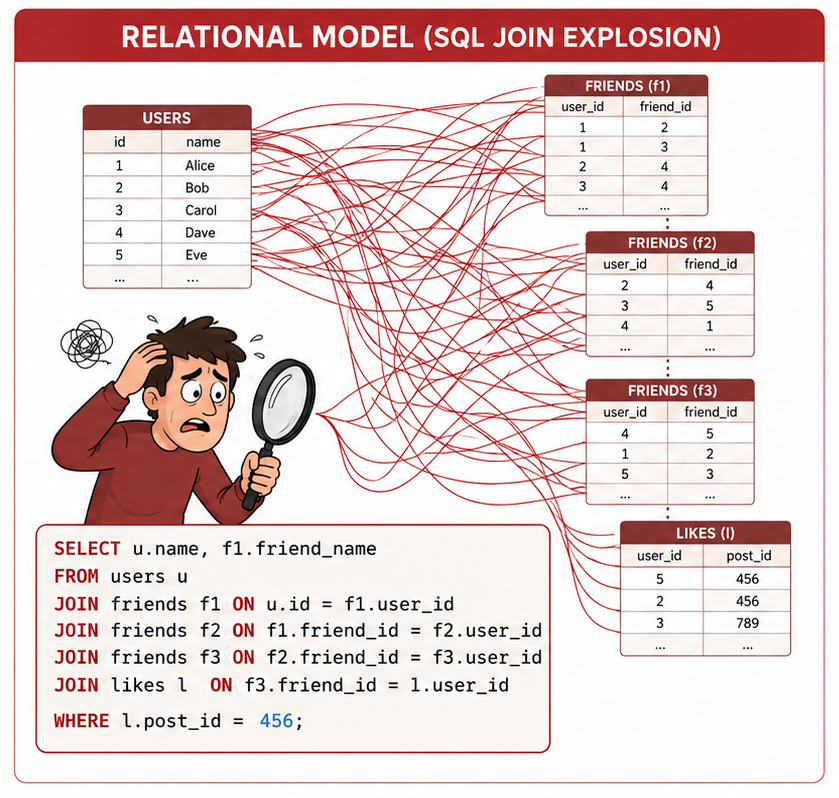
Complexity grows with depth

Depth	JOINs needed	Subqueries	Lines of SQL	Status
1 hop	1	0	~5	✓ Clean
2 hops	2	1	~12	Needs a comment
3 hops	3	2	~25	Requires explanation
N hops	N	N−1	O(N²)	Unmaintainable
Variable depth	?	?	?	Impossible without recursion

The database has no concept of "following a relationship."
Each JOIN is a full table scan or index lookup — computed fresh, every time.

Block 01 · The SQL "solution"

— recursive CTE (SQL:1999)

WITH RECURSIVE reachable AS (

  -- Base case: Alice's direct friends (depth 1)
  SELECT
    f.friend_id                    AS user_id,
    1                              AS depth,
    ARRAY[1, f.friend_id]          AS visited   -- track path to prevent cycles
  FROM friendships f
  WHERE f.user_id = 1

  UNION ALL

  -- Recursive case: follow one more hop
  SELECT
    f.friend_id,
    r.depth + 1,
    r.visited || f.friend_id
  FROM friendships f
  JOIN reachable r ON r.user_id = f.user_id
  WHERE f.friend_id != ALL(r.visited)   -- avoid cycles
    AND   r.depth < 3                      -- stop at depth 3

)
SELECT u.name, r.depth
FROM   reachable r
JOIN   users u ON u.id = r.user_id
WHERE  r.user_id != 1
ORDER BY r.depth, u.name;

This is the "clean" version — 20+ lines most developers can't write from memory.
Every detail (seed, cycle tracking, depth limit, start-node exclusion) is about how to traverse — not what data we want.
The business requirement is almost invisible in the code.

Block 01 · The SQL "solution"

Which databases support recursive queries?

Database	Support	Notes
PostgreSQL	✅ Full	Since v8.4 (2008). Cycle detection via `CYCLE` clause since v14
MySQL 8.0+	✅ Full	Since v8.0 (2018). Not in MySQL 5.x — still common in legacy
SQL Server	✅ Full	Max recursion depth defaults to 100 — set `OPTION (MAXRECURSION N)`
Oracle	✅ Full	Since 11g. Also has proprietary `CONNECT BY` syntax
SQLite	✅ Full	Since v3.8.3 (2014)
BigQuery	✅ Full	Added in 2022 — notably late for a major platform
Redshift	⚠️ Partial	Poor performance on deep recursion — not recommended for graph traversal
Hive / Spark SQL	❌ None	Workaround: iterative jobs or graph libraries (GraphX, GraphFrames)

01

Understanding

The depth-3 query no longer reads like a business requirement. Intent is buried under traversal mechanics.

02

Maintenance

Model change? Every depth level updates separately. No single place to change traversal logic.

03

Testing

Each depth is effectively a different query. Testing "the traversal" means N different SQL strings.

04

Performance

No concept of following a relationship — each JOIN is a fresh scan. At depth 3 over millions of users: timeouts.

The database isn't wrong. It's just not designed for this.

Block 01

01

Block 02

The graph data model —
from theory to property graph

Graph theory gives us the vocabulary. The property graph model adds what we need for real data: types and attributes.

02

Block 02 · Graph theory

G = (V, E)

A graph is an ordered pair of a set of vertices V and a set of edges E ⊆ V × V.
Edges connect two elements from V.

Type	What it means	Example
Directed	A→B ≠ B→A	"follows" on X
Undirected	A—B = B—A	"friends" on Facebook
Weighted	Edges carry a value	Road distances
Labelled	Nodes/edges carry type info	Property graph

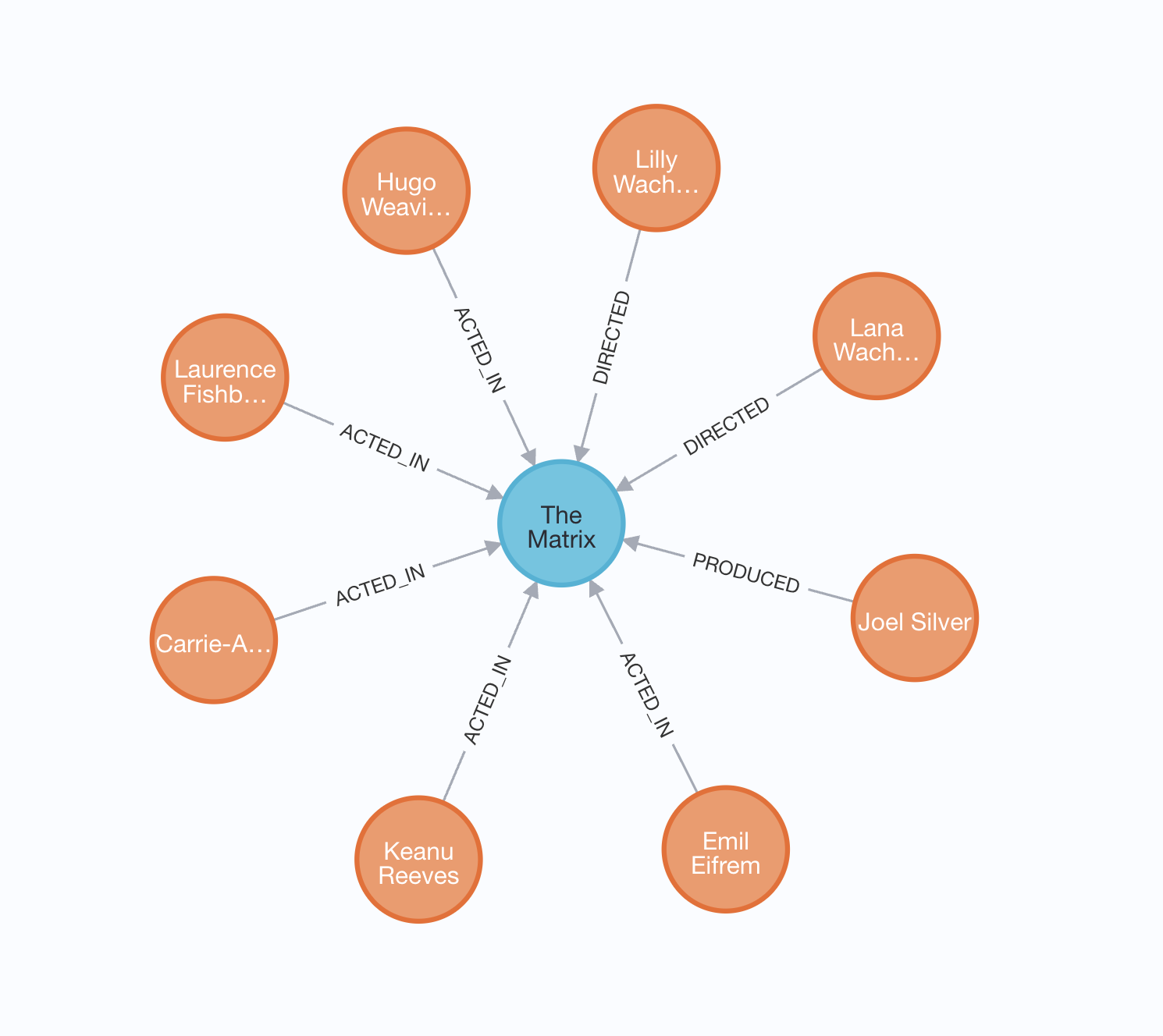
a directed labelled graph

Block 02 · Graph theory

Metro map, npm dependency tree, Wikipedia link graph.

All graphs.

You've been working with graph-structured data all along — just without the right tool.

Block 02 · Property graph model

Four concepts

Node — an entity (example: Person, account, device, IP).
Label — type tag on a node. A node can have multiple labels, e.g (:Client), (:Account).
Relationship — directed, typed, first-class.
Stored explicitly — not computed at query time.
Property — key-value pair on a node or relationship. That could be strings, numbers, booleans, dates, lists.

Key insight: relationships are physical data structures with direct pointers — not join results. This is why traversal is O(1) per hop.

a fraud detection subgraph

(:Client {name:"Anna", age:34}) │ │ [:OWNS {since:"2021-03"}] │ (:Account {id:"ACC-001", balance:5200}) │ │ [:TRANSFERRED_TO {amount:800}] │ (:Account {id:"ACC-002", balance:1100}) │ │ [:USES] │ (:IPAddress {value:"192.168.1.55"})

Block 02 · Same data, two models

Relational

clients
  (id, name, age)
accounts
  (id, client_id, balance)
transactions
  (id, from_account_id,
       to_account_id, amount, date)
ip_addresses
  (id, value)
account_ip
  (account_id, ip_id)

-- "Which clients share an IP?"
SELECT c1.name, c2.name, ip.value
FROM   clients c1
JOIN   accounts a1 ON a1.client_id = c1.id
JOIN   account_ip ai1 ON ai1.account_id = a1.id
JOIN   account_ip ai2 ON ai2.ip_id = ai1.ip_id
JOIN   accounts a2 ON a2.id = ai2.account_id
JOIN   clients c2 ON c2.id = a2.client_id
JOIN   ip_addresses ip ON ip.id = ai1.ip_id
WHERE  c1.id < c2.id;

Graph (property graph)

(:Client)-[:OWNS]->(:Account)
  -[:TRANSFERRED_TO]->(:Account)
(:Account)-[:USES]->(:IPAddress)

"Which clients share an IP?" — in Cypher

MATCH (c1:Client)-[:OWNS]->(a1:Account)
      -[:USES]->(ip:IPAddress)
      <-[:USES]-(a2:Account)
      <-[:OWNS]-(c2:Client)
WHERE c1.id < c2.id
RETURN c1.name, c2.name, ip.value

The query shape matches the data shape.
No junction tables. No computed joins.

Block 02 · The key technical insight

Index-free adjacency

Relational — JOIN

A relationship between two rows is discovered at query time by matching values. The database scans, compares, produces a result set. Fresh for every query.

Performance: O(log N) per hop — depends on index and table size.

Property Graph — pointer

A relationship is a physical pointer directly to the adjacent node. Traversing means following a pointer — one memory operation.

Performance: O(1) per hop — regardless of total DB size.
1M nodes = 1B nodes.

-- Friends within 3 hops — in Cypher (same line, any depth)
MATCH (:User {name:"Alice"})-[:FRIENDS_WITH*1..3]->(friend)
RETURN DISTINCT friend.name

Block 02 · Graph DB landscape

Three storage models

Model	Storage unit	Query lang
Property graph	Node + typed rel + props	Cypher, Gremlin
RDF / Triple store	Subject–Predicate–Object	SPARQL
Multi-model	Documents + graphs	AQL

RDF: semantic web, Wikidata, knowledge graphs — mention it so students recognise it. Focus stays on property graph — that's what the lab uses.

Neo4j — ACID & CAP

Fully ACID on single-instance and in cluster
Supports causal clustering for high availability
CAP position: CP — consistency + partition tolerance over availability
Transactions work as expected: BEGIN, execute Cypher, COMMIT or ROLLBACK

"Neo4j is not an eventually-consistent NoSQL store.
You get full transaction guarantees — critical for fraud detection."

Use a graph DB when…

Relationships are first-class data, not a side effect
Variable-depth traversals are common
Pattern matching across entities matters
Fraud detection, recommendations, knowledge graphs
Queries cross 3+ JOIN levels regularly

Stick with relational when…

Relationships are rare or structurally simple
Mostly aggregate queries: SUM, GROUP BY, reports
Strong ACID transactions are critical
Financial ledgers, structured CRUD, simple lookups

Graph DBs are a specialised tool, not a replacement for PostgreSQL.
Production systems may use both.

Block 03

Neo4j & Cypher —
live demo

Neo4j Browser open at localhost:7474

03

Block 03 · Cypher

SQL for graphs — read it like a picture

( )         a node
(:Label)    a node with a label
({k: v})    a node with a property
-->         directed relationship
-[:TYPE]->  typed relationship
-[:TYPE {k:v}]-> rel with properties

a full pattern

MATCH  (a:User)-[:FRIENDS_WITH]->(b:User)
WHERE  a.name = "Alice"
RETURN b.name

Block 03 · Cypher

Back to the friends-of-friends problem

With index-free adjacency, "friends of friends of friends" is just: follow a pointer, follow a pointer, follow a pointer.
The database does this natively, in a single pass, without scanning any tables.

MATCH (:User {name: "Alice"})-[:FRIENDS_WITH*1..3]->(friend)
RETURN DISTINCT friend.name;

One line. Change 3 to 6 — still one line. Change 3 to a variable — still one line.
No table scans. No JOINs. No cycle tracking. No depth management.
Just follow relationships.

Block 03 · Cypher syntax

The ASCII art is intentional.
Cypher was designed to be readable by someone who has never seen it before.

The query looks like the data it describes.

Block 03 · Cypher syntax · reading a pattern

"Find node a labelled User, connected via FRIENDS_WITH to node b labelled User, where a's name is Alice. Return b's name."

That's the whole query. Read left to right.

SQL — 1 hop (friends)

SELECT DISTINCT m.title
FROM   movies m
JOIN   watchings w  ON w.movie_id = m.id
JOIN   friendships f ON f.user_id_2 = w.user_id
JOIN   users u  ON u.id = f.user_id_1
WHERE  u.name = 'Alice'
  AND  m.id NOT IN (
    SELECT w2.movie_id
    FROM   watchings w2
    JOIN   users u2 ON u2.id = w2.user_id
    WHERE  u2.name = 'Alice'
  );

SQL — 2 hops (friends of friends)

SELECT DISTINCT m.title
FROM   movies m
JOIN   watchings w   ON w.movie_id = m.id
JOIN   friendships f1 ON f1.user_id_2 = w.user_id
JOIN   friendships f2 ON f2.user_id_2 = f1.user_id_1
JOIN   users alice   ON alice.id = f2.user_id_1
WHERE  alice.name = 'Alice'
  AND  m.id NOT IN (
    SELECT w2.movie_id FROM watchings w2
    JOIN   users u ON u.id = w2.user_id
    WHERE  u.name = 'Alice'
  );

Each extra hop = another JOIN + another subquery. SQL has no concept of depth.

Cypher — 1 hop

MATCH  (alice:Person {name: "Alice"})
       -[:FRIENDS_WITH]->(friend)
       -[:WATCHED]->(m:Movie)
WHERE NOT (alice)-[:WATCHED]->(m)
RETURN DISTINCT m.title

Cypher — 2 hops

MATCH  (alice:Person {name: "Alice"})
       -[:FRIENDS_WITH*1..2]->(friend)
       -[:WATCHED]->(m:Movie)
WHERE NOT (alice)-[:WATCHED]->(m)
RETURN DISTINCT m.title,
       count(friend) AS recommended_by
ORDER BY recommended_by DESC

*1..2 → *1..3. One token change.
The query reads like the business requirement — not the execution plan.

Block 03 · Demo

step 1 — basic MATCH and RETURN

// Find all clients
MATCH (c:Client)
RETURN c.id, c.name

SELECT * FROM clients — but we describe the shape of data, not the table name.
No schema declaration needed. Labels are flexible type tags, not rigid table definitions.

Block 03 · Demo

step 2 — follow a relationship

// Who owns which account?
MATCH  (c:Client)-[:OWNS]->(a:Account)
RETURN c.name, a.id, a.balance
ORDER BY a.balance DESC

No JOIN. The relationship is traversed directly — a pointer follow, not a table scan.
This is index-free adjacency in action: O(1) per hop.

Block 03 · Demo

step 3 — filter with WHERE

// Accounts with balance under 500
MATCH  (c:Client)-[:OWNS]->(a:Account)
WHERE  a.balance < 500
RETURN c.name, a.id, a.balance

WHERE works exactly like SQL — predicates on node and relationship properties.
The pattern in MATCH declares the shape; WHERE narrows the values.

Block 03 · Demo

step 4 — pattern matching

// Accounts that share an IP address — fraud signal
MATCH  (a1:Account)-[:USES]->(ip:IPAddress)
       <-[:USES]-(a2:Account)
WHERE  a1.id < a2.id  -- avoid duplicate pairs
RETURN a1.id, a2.id, ip.value AS shared_ip

Read the pattern: "account a1 uses an IP, and account a2 also uses the same IP."
We're asking the database to find a specific structural shape in the graph.
In SQL: 6 JOINs including a self-join on the junction table.

Block 03 · Demo

step 5 — variable-length traversal

// All accounts reachable within 3 transfer hops from ACC-001
MATCH  path = (:Account {id: 'ACC-001'})
              -[:TRANSFERRED_TO*1..3]->
              (b:Account)
RETURN b.id,
       length(path)               AS hops,
       [n IN nodes(path) | n.id]  AS chain

*1..3 — follow this relationship type between 1 and 3 times.
This is the query that required a recursive CTE in SQL. Here it's inline.
Change 3 to 10. The query is identical. No rewrite.

Block 03 · Demo

step 6 — shortest path

// Shortest transfer chain between two accounts
MATCH path = shortestPath(
  (:Account {id: 'ACC-001'})
  -[:TRANSFERRED_TO*]->
  (:Account {id: 'ACC-004'})
)
RETURN [n IN nodes(path) | n.id] AS chain,
       length(path)              AS hops

shortestPath() is a built-in function — not something you implement.
Neo4j knows it's a graph. The algorithm runs at the storage level, not application level.
Six degrees of separation — one MATCH clause.

Block 03 · Demo

step 7 — aggregation & hub detection

// Hub accounts — anomalously high incoming transfer count
MATCH  (src:Account)-[:TRANSFERRED_TO]->(hub:Account)
RETURN hub.id,
       count(src)        AS incoming_count,
       sum(src.balance)  AS total_incoming
ORDER BY incoming_count DESC

Equivalent to GROUP BY in SQL — but operating over a traversal result.
count(), sum(), avg(), collect() all work as expected.
Hub accounts with many incoming transfers = money laundering signal.

Block 03 · Cypher — quick reference

Clause	Purpose	SQL analogy
MATCH	Find a pattern in the graph	FROM + JOIN
WHERE	Filter on properties	WHERE
RETURN	Output columns	SELECT
CREATE	Create node or relationship	INSERT
MERGE	Create if not exists	INSERT … ON CONFLICT
SET	Update a property	UPDATE
DELETE / DETACH DELETE	Remove node or relationship	DELETE
WITH	Pipeline intermediate results	CTE
UNWIND	Expand a list into rows	UNNEST / LATERAL

Block 03 · Cypher

OPTIONAL MATCH
= LEFT JOIN

Regular MATCH works like INNER JOIN: if the pattern has no match, the row is dropped entirely.

If a person watched no movies — they disappear from the result.

MATCH (p:Person)-[:WATCHED]->(m:Movie)
Returns only people who watched something.
People with zero watches: not in results at all.

OPTIONAL MATCH — if pattern not found, variables are null.
The row stays. The person is there. The movie is null.

return everyone — null if no watches

MATCH (p:Person)
OPTIONAL MATCH (p)-[:WATCHED]->(m:Movie)
RETURN p.name, m.title

count watches — including zero

MATCH (p:Person)
OPTIONAL MATCH (p)-[:WATCHED]->(m:Movie)
RETURN p.name,
       count(m) AS watched_count
ORDER BY watched_count DESC

find people who never watched anything

MATCH (p:Person)
WHERE NOT (p)-[:WATCHED]->(:Movie)
RETURN p.name AS never_watched

Block 03 · OPTIONAL MATCH

Relationship must exist → use MATCH
Relationship may exist → use OPTIONAL MATCH

Same as INNER JOIN vs LEFT JOIN in SQL.

Block 03 · Cypher

WITH — pipeline between stages

WITH passes results from one stage to the next — like a Unix pipe or a SQL CTE.

Without it, you can't filter on aggregates.
This query fails:

// ERROR: can't use count() in WHERE directly
MATCH (p:Person)-[:FRIENDS_WITH]->(f)
WHERE count(f) > 2
RETURN p.name

WITH fixes it — aggregate first, then filter:

MATCH (p:Person)-[:FRIENDS_WITH]->(f)
WITH p, count(f) AS friends
WHERE friends > 2
RETURN p.name, friends
ORDER BY friends DESC

WITH for intermediate LIMIT — top 3 most connected, then find their movies

MATCH (p:Person)-[:FRIENDS_WITH]->(f)
WITH p, count(f) AS friends
ORDER BY friends DESC
LIMIT 3
MATCH (p)-[:WATCHED]->(m:Movie)
RETURN p.name, m.title, friends

WITH as a pipeline — step by step

MATCH … find data
WITH a, b, … choose what passes forward
(everything else is gone)
WHERE … filter the passed values
MATCH … continue with what remains
RETURN …

Analogy: if MATCH is FROM + JOIN, then WITH is a subquery you can keep building on — but it reads much cleaner.

Block 04 · Graph Data Science

"These aren't things you implement.
They're library calls on the graph you've already built."

Block 04 · Graph Data Science

Algorithms as library calls

Centrality: PageRank, Betweenness, Degree — "which nodes matter most?"
Community detection: Louvain, Label Propagation — "which nodes cluster together?"
Pathfinding: Dijkstra, A*, Yen's K-Shortest
ML on graphs: node2vec embeddings, Link Prediction, Node Classification

calling GDS from Cypher

// PageRank — find influential accounts
CALL gds.pageRank.stream('myGraph')
YIELD nodeId, score
RETURN gds.util.asNode(nodeId).id AS account,
       score
ORDER BY score DESC LIMIT 10

python integration

# Official Python driver
from graphdatascience import GraphDataScience
gds = GraphDataScience(uri, auth=(user, pwd))
results = gds.pageRank.stream(G)
# returns a Pandas DataFrame

Block 03 · context

When a graph DB is the wrong tool

Data is mostly flat. Event logs, sensor readings, order rows — almost no relationships. Graph adds zero value.
Queries are aggregations. "Total orders last month", "avg revenue by category" — SQL does this better, faster.
No traversal needed. You never ask "who is connected to X through Y" — you don't need a graph.
Very high write throughput. Neo4j is optimised for read traversal. Millions of events/sec → Kafka + ClickHouse.

Task	Right tool
Social graph, recommendations	Graph DB
Hierarchies, dependency trees	Graph DB
Fraud detection, routing	Graph DB
Reports, aggregations	PostgreSQL
Flat logs, time series	ClickHouse
Documents, flexible schema	MongoDB
Cache, sessions, counters	Redis

"Our shop has users, products, orders — that's a graph!" — technically yes. But if 90% of queries are flat lookups, PostgreSQL with two JOINs is the right answer.

Block 03 · NoSQL landscape

Where graph fits in NoSQL world

Type	Examples	Best for
Document	MongoDB, CouchDB	Semi-structured records
Key-value	Redis, DynamoDB	Caching, sessions
Column-family	Cassandra, HBase	Time series, write-heavy
Graph	Neo4j, FalkorDB	Connected data, traversals

Real systems combine all four

Redis — session caching, rate limiting
Cassandra — raw transaction event log
MongoDB — customer profiles, product catalog
Neo4j — relationship analysis, fraud patterns

FalkorDB — newer, runs inside Redis, uses sparse adjacency matrix (GraphBLAS). Supports Cypher. Significantly faster for high-throughput scenarios.
The graph DB space is actively evolving — more specialised engines for specific performance profiles.

Block 04

Industry context —
production graph databases

Real systems. Real queries. Where graph DBs earn their place in the stack.

04

Fraud detection

Mastercard · PayPal · HSBC

Fraud involves a network of actors — mule accounts, shared identities, layered transfers. Graph makes patterns visible instantly. Mastercard uses Neo4j to analyse transaction networks in real time, flagging ring structures and shared-credential clusters.

Recommendations

LinkedIn · Netflix

"People You May Know" = nodes 2 hops away you haven't connected to yet. Netflix finds content similarity paths via collaborative filtering. These queries run in milliseconds on graphs that would require many-table JOINs at scale.

Knowledge graphs

Google · Wikidata

Google's Knowledge Graph (the info panel in search results) connects entities through typed relationships. Wikidata: open knowledge graph with 100M+ items. Also: drug–target–disease graphs in pharma — fastest-growing use case.

up next · 90-minute lab

This is a lab preview. The full 90-minute hands-on session dives deeper into model design, CRUD operations, and query optimization.

Let's catch fraudsters

Task 1

Model design

Design the graph model from a raw dataset description. Define nodes, relationships, properties. No single right answer.

Task 2

CRUD operations

Load data with LOAD CSV. CREATE, MERGE, SET, DELETE. Merge duplicates. Basic data pipeline in Cypher.

Task 3

Analytical queries

Shared IP/device detection. Transfer chain traversal. Shortest path. Hub accounts. Bonus: equivalent SQL for the chain query.

"The hardest part is Task 1. Work backwards from the queries you'll need to run — let them drive the model design."